Replay and analysis interfaces

Analysis pipelines are external to this package. What it owes them is a stream whose contract is written down, and a way to develop against that stream without a market being open. This page is that contract.

The pipelines this was built to feed — exact waiting-time distributions of scalar series, long-memory estimation, criticality in tick arrival — live in separate packages of their own, not yet released. Nothing here depends on them, and the contract below is what any consumer gets. Two worked consumers ship under examples/, and the test suite executes both, so they cannot drift from what this page promises.

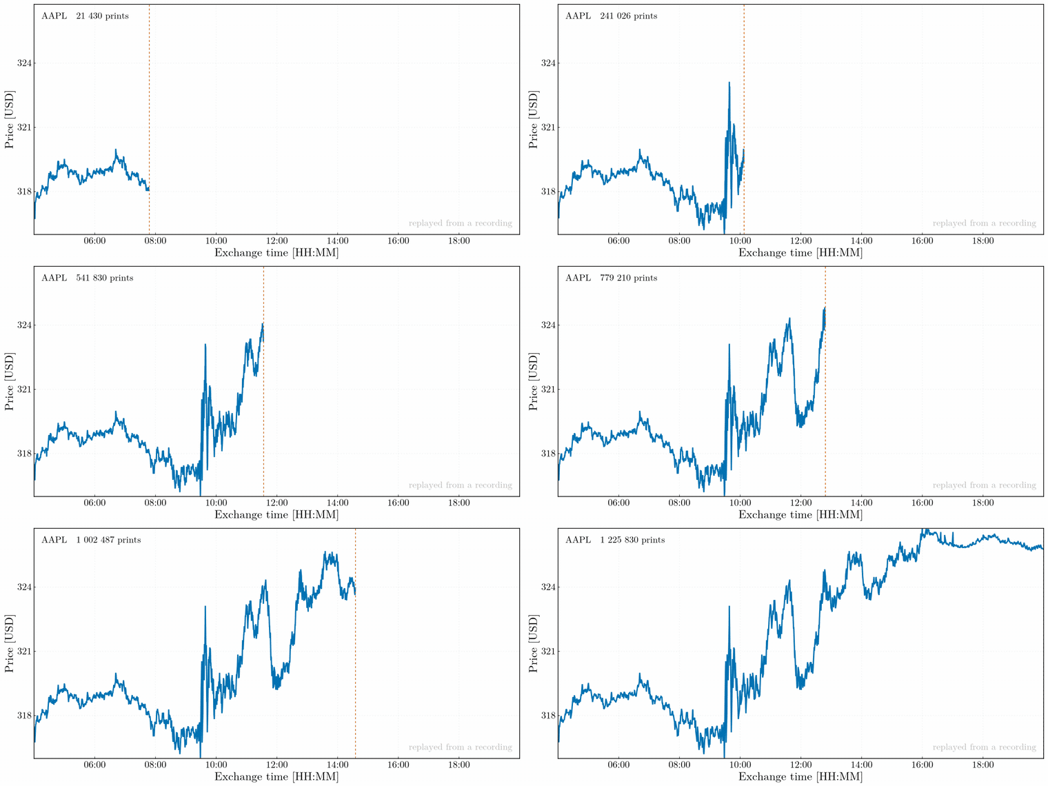
One interface, two sources

live_source and replay_source both hand back a Channel{Trade}. A consumer written against one works unchanged against the other, which is the point: a real-time method is developed and validated on recorded flux — reproducible, repeatable, free, available at three in the morning — and only then pointed at the wire.

using MarketTickStreamer

# Recorded session, re-emitted at the original inter-arrival times.
ch = replay_source("data/raw/session_part001.jsonl")

for trade in ch                      # terminates when the recording ends
    # ... the analysis method under test
end

pace = "max" drops the pacing and emits as fast as the consumer takes them, which is the mode for throughput work; speed compresses recorded time, so speed = 60.0 replays an hour of tape in a minute.

A session is replayed from its raw files, which are read whole. A corpus is replayed from the processed tree, and streamed: the files of one trading day — one per symbol — are loaded, merged on the clock and emitted before the next day is opened, so a symbol-year replays in the memory of its busiest day.

files = processed_files("data/processed", "AAPL"; from = Date(2026, 5, 1))
for trade in replay_source(files; pace = "max")
    # ... an estimator run over months of tape
end

Six AAPL days, 5.6 million prints, go through at about a million prints per second with the resident set flat at 1.2 GiB from the first day to the last. Recorded pace keeps one schedule across the days, closures included, so replaying a week at speed = 1 takes a week. If a later day cannot be read, the channel closes with that error and the consumer's loop rethrows it, after every earlier print has been delivered.

What a Trade means

Two clocks per print is a deliberate choice: with time_ns and recv_ns both recorded, feed latency is a measurable quantity afterwards rather than an assumption baked in at capture time.

Trade carries value semantics — == and hash compare fields, not the identity of the conditions vector — so round-tripping through the raw layer produces objects that compare equal.

Guarantees

Ordering. Replay emits in ascending order of its clock, sorted on load: recv_ns when every record carries one, time_ns otherwise (clock = "auto"; either can be forced). Backfilled records have recv_ns = 0, so a backfilled recording replays on exchange time.

Pacing. Each emission is scheduled against the absolute time elapsed since the first record, not slept gap by gap. sleep overshoots by about a millisecond, so per-gap sleeping stretches a session whose gaps are of that order — 65 % on gaps of 2.5 ms — whereas on an absolute schedule the error stays within one overshoot however long the replay runs. Gaps below a millisecond are emitted back to back, in order. The live source emits in arrival order, which is not the same as ascending time_ns: a consolidated tape interleaves venues, and late prints are normal. Any method that needs monotone exchange time must sort or reject explicitly; session_report quantifies how often it happens in a given capture.

Completion. Both sources close the channel when the stream ends — the recording exhausted, the session deadline reached, the market closed, a fatal protocol error. A for t in ch loop therefore terminates on its own, and a consumer needs no separate shutdown signal.

Backpressure. The channel is bounded (limits.channel_capacity). A slow consumer blocks the producer, and on a live session that propagates into TCP backpressure rather than into unbounded memory growth. This is why the default is to block: silently dropping ticks would corrupt exactly the arrival statistics the package exists to measure.

Determinism. Replaying the same files with pace = "max" yields the identical sequence every time. With pace = "recorded" the sequence is identical but the timing is approximate: gaps under a millisecond are not resolvable by sleep, so they are emitted back to back.

Fanning out to several consumers

tee splits one stream into independent channels, with a per-output overflow policy:

session = live_source(provider, cfg)
persist, analyse = tee(session.channel, 2; lossy = [false, true])

A non-lossy output blocks the fan-out when full — use it for persistence, which must always win. A lossy output drops incoming ticks instead of stalling the capture, counts the drops, and reports them through on_drop. An analysis tap that occasionally cannot keep up belongs on a lossy output; one whose results depend on seeing every print does not, and should instead run offline against the raw files, where nothing is ever dropped.

A worked consumer

examples/waiting_times.jl is this page in code: it replays a recorded session, splits it with tee into a lossless consumer and a lossy analysis tap, accumulates inter-arrival times in a single pass, and stops when the channel closes — no shutdown protocol of its own.

julia examples/waiting_times.jl data/raw/<session>_part001.jsonl

It reports both populations side by side, which is the cheapest way to see what the choice costs on your own data. One AAPL session, 1 225 831 prints:

every execution          n=  1225830  mean=  0.0470 s  median=  0.0007 s  p99=  0.6231 s  max=   30.080 s
price-forming only       n=   408793  mean=  0.1409 s  median=  0.0005 s  p99=  1.4756 s  max=  116.269 s

A median of 0.7 ms against a mean of 47 ms is the distribution announcing itself. Note also that excluding odd lots raises the mean roughly threefold while leaving the median where it was: it thins the dense clusters and stretches the tail rather than rescaling the whole distribution.

Both tee outputs in the example are lossless, deliberately. At maximum replay rate a lossy tap lost 85 000 of those prints — and it does not thin a sample evenly, it removes the bursts, which is where a waiting-time distribution lives. Backpressure costs nothing offline, since a blocked output only slows the replay.

The suite executes the example, so it cannot drift from the interface it documents.

Which prints count as trades

conditions is reported, never acted on at capture. Whether a print belongs in your sample depends on the question, and the two questions this package serves want opposite answers:

• A price path — returns, volatility, Hurst or DFA estimation — wants price-forming prints only. Odd lots, contingent and derivatively priced trades and corrections carry prices that were never a consolidated last sale, and differencing them manufactures volatility nobody could trade on.
• An arrival process — waiting-time distributions, tick intensity, criticality — wants every execution. An odd lot is a real fill by a real participant at a real instant, and dropping it distorts the very law under study.

So price_forming and filter_price_forming operate on loaded prints, and session_report reports n_trades beside n_price_forming so the size of the distinction is measured per capture rather than assumed. The gap is dominated by odd lots and grows with share price, so it varies strongly across a basket.

The default population, NON_PRICE_CONDITIONS, follows the tape plans' own sale-condition matrices: a code is excluded when the plan does not let it update the consolidated last sale, or lets it only when it is the sole qualifying trade of the day. That takes out odd lots, average-price prints (B on tapes A and B, W on tape C), prices fixed earlier or elsewhere (P, 4), late reports (Z, U), contingent trades and non-regular settlement. Extended-hours prints (T) stay in, because at tick resolution they are the price path of their session. Average-price and derivatively priced prints are few — about 3 % of what otherwise passes on a liquid Nasdaq name — but they are the ones that land percents away from the market: on one AAPL session they moved the day's price-forming minimum from 316.00 to 304.35. The lists are configuration ([quality.non_price_conditions]), so the population a session was reported under is recorded in its sidecar.

State which of the two populations a result used. After the fact, a price series does not reveal it.

Sampling on a clock that runs with the market

Market activity is not uniform in time, so sampling a price path every minute draws unevenly from the process that generates it — densely at the open, sparsely at lunch. tick_bars, volume_bars and dollar_bars resample a capture onto clocks that advance with activity instead: one bar per fixed count of prints, of shares, or of traded value.

trades = read_raw(files)
bars = dollar_bars(filter_price_forming(trades), 5.0e6)   # one bar per $5M traded

The empirical motivation is old and well tested: price changes sampled in transaction time are far closer to independent and normal than calendar-time changes (Mandelbrot & Taylor 1967; Clark 1973; Ané & Geman 2000). Of the three, the value clock is the one that survives a change of scale — it is invariant to splits and roughly invariant to price drift, so a threshold chosen on one sample still means something on another.

Two choices are yours and are not incidental. Whether to filter to price-forming prints first changes the bar count by a factor of three on a high-priced name. And the bars carry recv_ns = 0, the same marker the raw layer uses for records that never crossed the wire, because a derived bar has no receipt time.

A Bar records both ends of its interval: time_ns is the timestamp of its first print and close_ns that of the print that completed it. On an activity clock the amount transacted per bar is fixed and the duration is what varies, so close_ns - time_ns is itself a waiting time — that of a fixed quantity of activity rather than of a single print:

durations_s = [(b.close_ns - b.time_ns) / 1e9 for b in bars]

Consecutive bars never overlap, bars[i].close_ns <= bars[i+1].time_ns, and the gap between them is the wait for the next bar's first print.

Working from the file layer instead

For methods that need the whole record rather than a stream — tail exponents, long-memory estimation, anything needing the sample in memory — read_raw returns a Vector{Trade} from raw NDJSON, and compact_raw writes per-symbol per-day CSV or Arrow that any other tool can read. The raw layer is the source of truth; compaction is a convenience over it, never a replacement.